Support Vector Machines & Gradient Descent
In this post, I will discuss Linear SVM using Gradient Descent along with Platt scaling

Photo by Charles Deluvio on Unsplash
This is part 3 of my post on Linear Models. In part 1, I had discussed Linear Regression and Gradient Descent and in part 2 I had discussed Logistic Regression and their implementations in Python. In this post, I will discuss Support Vector Machines (Linear) and its implementation using Gradient Descent.
Introduction :
Support-vector machines (SVMs) are supervised learning models capable of performing both Classification as well as Regression analysis. Given a set of training examples each belonging to one or the other two categories, an SVM training algorithm builds a model that assigns new examples to one category or the other. SVM is a non-probabilistic binary linear classification algorithm ie given a training instance, it will not output a probability distribution over a set of classes rather it will output the most likely class that the observation should belong to. However, methods such as Platt scaling exist to use SVM in a probabilistic classification setting. Platt scaling or Platt Calibration is a way of transforming the outputs of a classification model into a probability distribution over classes. Platt scaling works by fitting a logistic regression model to a classifier’s scores. In addition to performing linear classification, SVMs can efficiently perform a non-linear classification using what is called the kernel trick, implicitly mapping the inputs into high-dimensional feature spaces. In the case of support vector machines, a data point is viewed as a p−dimensional vector(a list of p numbers), and we want to know whether we can separate such points with a (p−1)-dimensional hyperplane. There are many hyperplanes that might classify the data. One reasonable choice as the best hyperplane is the one that represents the largest separation, or margin, between the two classes. So we choose the hyperplane so that the distance from it to the nearest data point on each side is maximized. Such a hyperplane is called as a maximum-margin hyperplane and the linear classifier it defines is called as a margin maximizing classifier.
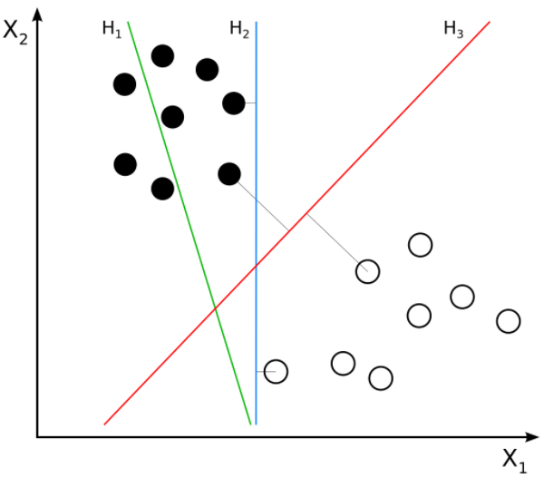
Source: Wikipedia
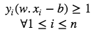
Here we can see three hyperplanes H1, H2, H3. Here H1 does not separate the classes, but H2 and H3 do but the margin is maximum for H3. A good separation is achieved by the hyperplane that has the largest distance to the nearest training-data point of any class. The larger the margin, the lower the generalization error of the classifier. Consider we are given the following training examples :
Here each yi belongs to either +1 or -1 indicating the class to which yi belongs to. and each xi is a p-dimensional real vector. The objective is to find a hyperplane that maximises the margin that divides the group of data points xi for which yi = 1 and for which yi = −1.
Any hyperplane can be written as the set of points x satisfying:

Where w is the normal vector to the hyperplane. Here w need not be normalized. The parameter (b/||w||) determines the offset of the hyperplane from the origin along the normal vector w.
Hard Margin SVM
If the data is linearly separable, we can select two parallel hyperplanes that separate the two classes of data, so that the distance between them is as large as possible. The region bounded by these two hyperplanes is called the margin, and the maximum-margin hyperplane is the hyperplane that lies halfway between them. These hyperplanes can be described with the following equations :

Anything on or above this boundary is of class with label 1
Anything on or below this boundary is of the class with label −1
Geometrically the distance between these two hyperplanes is given as (2/||w||), so to maximize the distance between the planes, we want to minimize ||w|| The distance is computed using the distance from a point to a plane equation. To prevent data points from falling into the margin, we add the following constraint: for each i either:


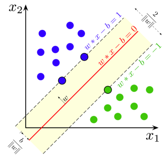
Source: Wikipedia
These constraints state that each data point must lie on the correct side of the margin. The above constraints can be rewritten as:
The optimization problem can be written as :
The w and b that solve this problem determine the classifier. Given an input x, the model’s output is given by:
Maximum-margin hyperplane is completely determined by those xi which is nearest to it. These xi are called Support vectors. ie they are the data points on the margin.
Soft-margin SVM
Hard-margin SVM requires data to be linearly separable. But in the real-world, this does not happen always. So we introduce the hinge-loss function which is given as :

This function outputs 0, if xi lies on the correct side of the margin. For data on the wrong side of the margin, the function’s value is proportional to the distance from the margin. Here we need to minimize the following :

λ determines the tradeoff between increasing the margin size and ensuring that the xi lie on the correct side of the margin. For sufficiently small values of λ , the second term in the loss function will become negligible, hence, it will behave similar to the hard-margin SVM.
Computing the SVM classifier
Primal :
Minimizing the above equation can be rewritten as a constrained optimization problem with a differentiable objective function in the following way :
For each i∈{1,….,n}, we introduce a variable ζ(Zeta), such that :

ζ is the smallest nonnegative number satisfying :
Now we can rewrite the optimization problem as :

The Dual :
Even though we can solve the primal using Quadratic Programming(QP), solving the dual form of the optimization problem plays a key role in allowing us to use kernel functions to get the optimal margin classifiers to work efficiently in very high dimensional spaces. The dual form will also allow us to derive an efficient algorithm for solving the above optimization problem that will typically do much better than generic QP. By solving for the Lagrangian dual of the above problem, we can get the simplified problem :
αi is defined such that:

It follows that w can be written as a linear combination of the support vectors. The offset, b, can be recovered by finding an xi on the margin’s boundary and solving the following :
Kernel trick :
This is used to learn a nonlinear classification rule by projecting the non-linear dataset into a higher dimensional space in which the data is linearly separable. Here we apply a function called the Kernel Function, which maps the data into higher dimensional space where the data is linearly separable. Let us denote the transformed data points as φ(xi) and we have a kernel function K which satisfies the following :
Some of the common Kernels are as follows :
- Polynomial Kernel: For degree-_d_ polynomials, the polynomial kernel is defined as :
If c=0, then the Kernel is called Homogeneous
- Gaussian Radial Basis Function :
- Hyperbolic tangent :

The classification vector w in the transformed space satisfies :
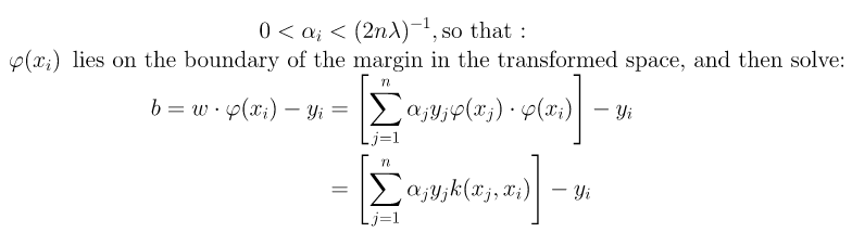
Where αi is obtained by solving the optimization problem :
We can solve αi using techniques such as Quadratic Programming, Gradient Ascent or using Sequential Minimal Optimization(SMO) techniques. We can find some index i such that :
So for a new datapoint z, we can get the class it belongs to using the following:

Sub-Gradient Descent for SVM
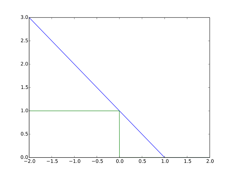
As mentioned earlier, linear SVM use hinge-loss, the below plot is a comparison between 0–1 loss and the hinge-loss :
Source: Wikipedia
Here the Blue is the Hinge Loss and Green is 0–1 loss. Why can’t we use 0–1 Loss in SVM instead of Hinge Loss?
0–1 loss function is flat so it doesn’t converge well. Also, it is not differentiable at 0. SVM is based on solving an optimization problem that maximize the margin between classes. So in this context, a convex loss function is preferable so we can use several general convex optimization methods. The 0–1 loss function is not convex so it is not very useful either. SVM objective function is nothing but Hinge loss with l2 regularization :

This function is not differentiable at x=1. The derivative of hinge loss is given by:

We need gradient with respect to parameter vector w. For simplicity, we will not consider the bias term b.


So the Gradient of SVM Objective function is :


Subgradient Of SVM Loss Function :


So the Subgradient of Cost Function can be written as :

SVM Extensions :
- Multiclass SVM :
SVM is a binary classifier and hence directly it doesn’t support multiclass classification problem. So one way of dealing with multiclass setting is to reduce the single multiclass problem into multiple binary classification problems. One method to do this is to binary classifiers that distinguish between one of the labels and the rest (one-versus-all) or between every pair of classes (one-versus-one). One-versus-all is done by done by a winner-takes-all strategy in which the classifier with the highest output function is assigned the class, here the output functions must be calibrated to produce comparable scores. In one-versus-one classification is done by a max-wins voting strategy, in which every classifier assigns the instance to one of the two classes, then the vote for the assigned class is increased by one vote, and finally the class with the most votes determines the instance classification.
- Support Vector Regression :
Training an SVR(Support Vector Regressor) means solving the following :


where xi is the training sample and yi is the target value. Here ϵ is the parameter that serves as a threshold ie all the predictions have to be within ϵ range of true predictions.
Platt Scaling :
In machine learning, Platt scaling or Platt calibration is a way of transforming the outputs of a classification model into a probability distribution over classes. Platt scaling works by fitting a logistic regression model to a classifier’s scores. Consider that we have a binary classification problem: So for a given input x, we want to determine if they belong to either of two classes +1 or −1. Let’s say the classification problem will be solved by a real-valued function f, by predicting a class label y=sign(f(x)). Platt Scaling produces probability estimates by applying a logistic transformation of the classifier scores f(x) :

The parameters A and B are estimated using maximum likelihood estimation from the training set (fi,yi). First, let us define a new training set (fi,ti)where ti are target probabilities defined as :

The parameters A and B are found by minimizing the negative log likelihood of the training data, which is a cross-entropy error function :


The minimization is a two-parameter minimization. Hence, it can be performed using any number of optimization algorithms. The probability of correct label can be derived using Bayes’ rule. Let us choose a uniform uninformative prior over probabilities of correct label. Now, let us observe that there are N+ positive examples and N- negative examples. The MAP estimate for the target probability of positive examples(y=+1) is :

The MAP estimate for the target probability of negative examples(y=−1)(y=−1) is :

These targets are used instead of {0, 1} for all of the data in the sigmoid fit. These non-binary targets value are Bayes-motivated and these non-binary targets will converge to {0,1} when the training set size approximates to infinity, which recovers the maximum likelihood sigmoid fit.
Now let us implement linear SVM for a binary classification using the Sub-Gradient Descent which I have described above :
Let us create a simple dataset :
X = np.random.rand(1000,2)
y = 2 * X[:, 0] + -3 * X[:, 1]
y = np.round(1/(1 + np.exp(-y)))

for i in range(len(y)):  #Changing labels from [0,1] to [-1,+1]
    if(y[i]==0):
        y[i] = -1
    else:
        y[i] = 1
Now let us plot the data :
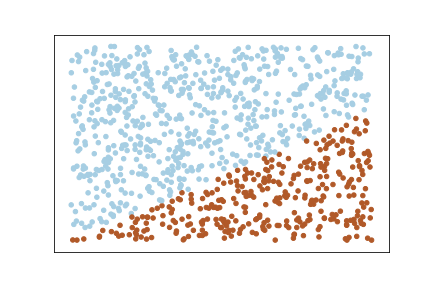
Here we can see that the data is linearly separable, but at the same time the margin size should be very small. If we increase the margin here, then the misclassifications will more.
Now let’s define the hinge loss function :
def hinge_loss(x, y, w, lambdh):
    b = np.ones(x.shape[0]) #Intercept term: Initialize with ones.
    distances = 1 - y * (np.dot(x, w)-b)
    distances[distances < 0] = 0  # equivalent to max(0, distance)
    loss = np.sum(distances) / x.shape[0]

    # calculate cost
    hinge_loss = lambdh * np.dot(w, w) + loss

    return hinge_loss
Now let’s define the function to get the gradients of hinge loss :
def get_grads(x,y,w,lambdh):
    b = np.ones(x.shape[0]) #Intercept or Bias: Initialize with ones
    grad_arr = []
    I = y * (np.dot(x, w)-b)  #Indicator Function

    for i in range(len(I)):
        if(I[i]<1):
            I[i] = 1
        else:
            I[i] = 0

    for i in range(x.shape[0]):
        grad_arr.append(-y[i]*x[i]*I[i])

    grads = np.sum(grad_arr, axis=0)/x.shape[0] + 2*lambdh*w
    return grads
Mini-Batch SGD :
w = np.array([1,-6]) #Initial Weights
eta= 0.1 # learning rate
n_iter = 1000 # Number of Iterations
batch_size = 128
loss = np.zeros(n_iter) #Array to store loss in each iteration
lambdh = 0.001  #To control the margin width.

for i in range(n_iter):
    ind = np.random.choice(X.shape[0], batch_size)
    loss[i] = hinge_loss(X[ind, :], y[ind], w, lambdh)
    w = w - eta * get_grads(X[ind, :], y[ind], w, lambdh)
Here you can change the value of ‘lambdh’ parameter and see the model’s performance. If you increase the margin size, it can be observed that the number of misclassifications increase.
SGD With Momentum :
w = np.array([1,-6]) #Initial Weights
eta = 0.05 # learning rate
alpha = 0.9 # momentum

h = np.zeros_like(w)  #This is an additional vector
es = 0.0001 #For early stopping
n_iter = 1000 #Number of iterations

batch_size = 128
lambdh = 0.001
loss = np.zeros(n_iter) #List to store the loss in each iteration

for i in range(n_iter):
    ind = np.random.choice(X.shape[0], batch_size)
    loss[i] = hinge_loss(X[ind, :], y[ind], w, lambdh)

    h = alpha * h + eta * get_grads(X[ind, :], y[ind], w, lambdh)
    w = w-h
SGD With Nestrov accelerated momentum :
w = np.array([1,-6]) #Initial Weights
eta = 0.05 # learning rate
alpha = 0.9 # momentum

h = np.zeros_like(w)  #This is an additional vector
es = 0.0001 #For early stopping

n_iter = 1000 #Number of iterations
batch_size = 128
lambdh = 0.001 #To control the width of the margin
loss = np.zeros(n_iter) #List to store the loss in each iteration

for i in range(n_iter):
    ind = np.random.choice(X.shape[0], batch_size)
    loss[i] = hinge_loss(X[ind, :], y[ind], w, lambdh)

    h = alpha * h + eta * get_grads(X[ind, :], y[ind], w, lambdh)
    w = w-h
RMSProp :
w = np.array([1,-6]) #Initial Weights
eta = 0.05 # learning rate
alpha = 0.9 # momentum

gt = None
eps = 1e-8
es = 0.0001 #For early stopping

lambdh = 0.001
n_iter = 1000
batch_size = 128
loss = np.zeros(n_iter)

for i in range(n_iter):
    ind = np.random.choice(X.shape[0], batch_size)
    loss[i] = hinge_loss(X[ind, :], y[ind], w, lambdh)

    gt = get_grads(X[ind, :], y[ind], w, lambdh)**2
    gt = alpha * gt +(1-alpha) * gt

    a = eta * get_grads(X[ind, :], y[ind], w, lambdh)np.sqrt(gt+eps)
    w = w-a
Adam :
w = np.array([1,-6]) #Initial Weights
eta = 0.05 # learning rate
alpha = 0.9 # momentum

gt = None
vt = 0
beta = 0.0005

eps = 1e-8
es = 0.1 #For early stopping
lambdh = 0.001

n_iter = 1000
batch_size = 128
loss = np.zeros(n_iter)

for i in range(n_iter):
    ind = np.random.choice(X.shape[0], batch_size)
    loss[i] = hinge_loss(X[ind, :], y[ind], w, lambdh)

    gt = get_grads(X[ind, :], y[ind], w, lambdh)**2
    vt = (beta*vt) + (1-beta)*gt

    a = eta * get_grads(X[ind, :], y[ind], w, lambdh)/np.sqrt(vt)+eps
    w = w-a
Platt Scaling :
The following implementation is based on the paper published by Platt which is available here.
def platt_calib_parms(out,target,prior1,prior0):
    #out = array of SVM outputs
    #target = array of booleans: is ith example a positive example?
    #prior1 = number of positive examples
    #prior0 = number of negative examples
    A = 0
    B = np.log((prior0+1)/(prior1+1))
    hiTarget = (prior1+1)/(prior1+2)

    loTarget = 1/(prior0+2)
    lambdah = 1e-3
    olderr = 1e300

    pp = np.zeros(prior0+prior1)      # temp array to store urrent estimate of probability of examples

    for i in range(len(pp)):
        pp[i] = (prior1+1)/(prior0+prior1+2)

    count = 0
    for it in range(1,100):
        a = 0
        b = 0
        c = 0
        d = 0
        e = 0
        #compute Hessian & gradient of error funtion with respet to A & B
        for i in range(len(target)):
            if (target[i]==1):
                t = hiTarget
            else:
                t = loTarget
            d1 = pp[i]-t
            d2 = pp[i]*(1-pp[i])
            a += out[i]*out[i]*d2
            b += d2
            c += out[i]*d2
            d += out[i]*d1
            e += d1
        #If gradient is really tiny, then stop
        if (abs(d) < 1e-9 and abs(e) < 1e-9):
            break
        oldA = A
        oldB = B
        err = 0

        #Loop until goodness of fit inreases

        while (1):
            det = (a+lambdah)*(b+lambdah)-c*c
            if (det == 0):  #if determinant of Hessian is zero,inrease stabilizer
                lambdah *= 10
                ontinue
            A = oldA + ((b+lambdah)*d-c*e)/det
            B = oldB + ((a+lambdah)*e-c*d)/det

            #Now, ompute the goodness of fit
            err = 0
            for i in range(len(target)):
                p = 1/(1+np.exp(out[i]*A+B))
                pp[i] = p

                #At this step, make sure log(0) returns -200
                err -= t*np.log(p)+(1-t)*np.log(1-p)

            if (err < olderr*(1+1e-7)):
                lambdah *= 0.1
                break
            #error did not derease: inrease stabilizer by fator of 10 & try again
            lambdah *= 10
            if (lambdah >= 1e6):  # Something is broken. Give up
                break
            diff = err-olderr
            sale = 0.5*(err+olderr+1)
            if (diff > -1e-3*sale and diff < 1e-7*sale):
                count+=1
            else:
                count = 0
            olderr = err
            if(count==3):
                break
    return A,B
The code will return the parameters A and B. Now to get the probabilities :
target = y #True Labels
out = y_predicted #Predicted Labels

prior1 = len(y[y==1]) #Number of positive samples
prior0 = len(y[y==-1]) #Number of negative samples
A,B = platt_calib_parms(target,out,prior1,prior0)

#Once we obtain A and B then :
#Probability that a datapoint belongs to Positive class :
p_pos = 1/(1+np.exp(A * out+B))

#Probability that a datapoint belongs to Negative class :
p_neg = 1-p_pos
The full implementation along with the results and plots are available here. In this implementation, I haven’t tested the results with that of Sklearn Implementation and the above dataset is created only for learning purpose and in real-world data will not be like this and you might have to do preprocessing before applying Machine Learning Models.
References :
- https://davidrosenberg.github.io/mlcourse/Archive/2018/Lectures/03c.subgradient-descent.pdf
- https://en.wikipedia.org/wiki/Support_vector_machine
- http://acva2010.cs.drexel.edu/omeka/items/show/16561
- https://alex.smola.org/papers/2003/SmoSch03b.pdf
- http://citeseerx.ist.psu.edu/viewdoc/download;jsessionid=4DDE09F156D9C7B25755CE1B2B593F2F?doi=10.1.1.41.1639&rep=rep1&type=pdf
- https://people.eecs.berkeley.edu/~jordan/courses/281B-spring04/lectures/lec3.pdf
- https://svivek.com/teaching/lectures/slides/svm/svm-sgd.pdf
- https://www.youtube.com/watch?v=jYtCiV1aP44
- https://www.youtube.com/watch?v=vi7VhPzF7YY