Logistic Regression & Gradient Descent
This is Part 2 of my Posts on Linear Models. In Part 1, I have discussed about Linear Regression as well as Gradient Descent. For Part 1 please click here

Photo by Drew Graham on Unsplash
Introduction :
Logistic Regression is also called as Logit Regression is used to estimate the probability that an instance belongs to a particular class(eg: the probability that it rains today?). If the estimated probability is greater than 50%, then the model predicts that the instance belongs to that class(positive class labelled “1”) or else it predicts the probability it does not belong to that class(ie the probability it belongs to negative class labelled “0”). Just like Linear Regression, a Logistic regression also computes a weighted sum of input features(plus a bias), but instead of outputting the result directly like Linear regression model does, it outputs the Logistic of this result :

The logistic also called the logit, noted as σ(.) is a sigmoid function which takes a real input and outputs a value between 0 and 1.
A graph of the logistic function on the t-interval (−6,6) is given below:
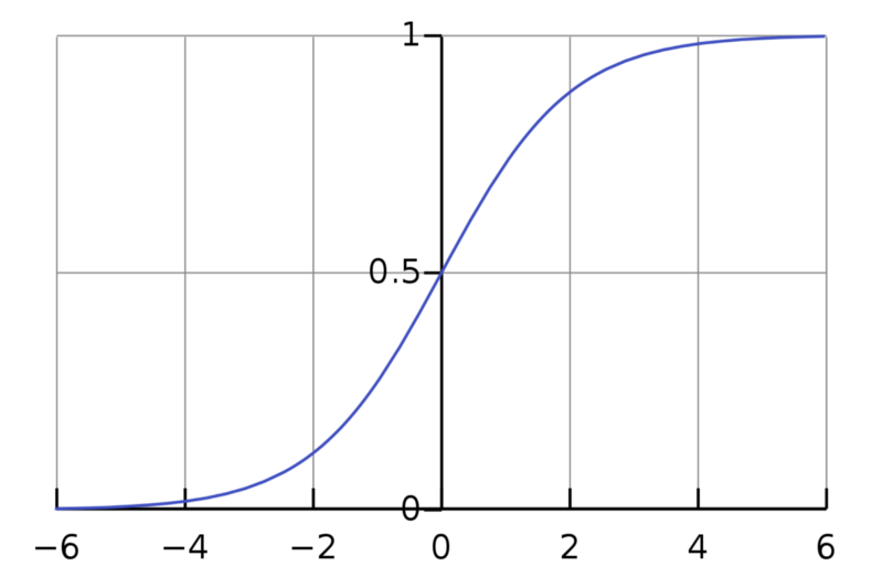
Source : Wikipedia
Once the Logistic Regression model has estimated the probability p̂ , the model can make predictions using :
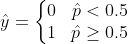
σ(t)<0.5 when t<0 and σ(t)≥0.5 when t≥0 , ie Logistic Regression predicts 1 when :
And predicts 0 when it is negative.
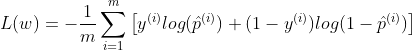
Loss Function :
The objective of training is to set the parameter vector w so that the model predicts high probability for positive class(y=1) and low probabilities for negative instances(y=0). For a single training instance x, the loss function can be given as :
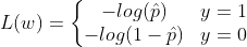
−log(t) grows very large when t approaches 0, so the cost will be large if the model estimates a probability close to 0 for a positive instance and it will also be very large if the model estimates a probability close to 1 for a negative instance.
−log(t) is close to 0 when t is close to 1, so the cost will be close to 0 if estimated probability is close to 0 for a negative instance or close to 1 for a positive instance, which is exactly what we need.
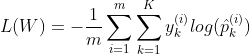
The loss function over the whole training set is simply the average loss over all training instances:
Unlike the Linear Regression, there is no closed form/normal equation to find the value of w that minimizes the loss function. But the function is convex one, so Gradient Descent or any other optimization algorithm is guaranteed to find the global minimum. You can read about Gradient Descent in my post on Linear Regression and Gradient Descent.
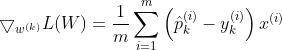
The partial derivative of the loss function with respect to the jth model parameter wj is given by:
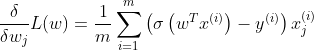
For each instance it computes the prediction error and multiplies it by the jth feature value and then it computes the average over all training instances. Once we get the gradient vector containing all the partial derivatives, we can use it in the GD/SGD/mini-batch SGD.
Softmax Regression :
Logistic Regression can be generalized to support multiple classes directly without having to train and combine multiple binary classifiers. This is called as Softmax Regression or Multinomial Logistic Regression.
When given an instance x, the Softmax Regression model first computes a score(z) for each class k, then estimates the probability of each class by applying a softmax function.
The equation to calculate the softmax score for class k is given by:
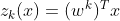
Each class has a parameter vector w. All these are typically stored as rows in a parameter matrix W. After computing the score for every class for the instance x, we can estimate the probability that the instance belong to class k by running the scores through the softmax function. Which is given below as:
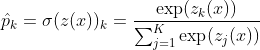
The softmax function computes the exponential of every score and then normalizes them by dividing by the sum of all the exponents. K is the total number of classes. z(x) is a vector containing the scores of each class for the instance x. σ(z(x))k is the estimated probability that the instance x belongs to the class k given the scores of each class for that instance. Like Logistic Regression classifier, the Softmax Regression classifier predicts the class with the highest estimated probability(which is simply the class with the highest score):

The Softmax regression only predicts one class at a time(it is multiclass not multioutput), so it should only be used with mutually exclusive classes such as different types of plants. You cannot use it to recognize multiple people in one picture. The objective is to have a model that estimates high probability for the target class and low probability for the other class. So for this we need to minimize the cross entropy loss which penalizes the model when it estimates a low probability for a target class.
y is equal to 1, if the target class for the ith instance is k; otherwise it is equal to 0. When there is two classes (K=2), the loss function is equivalent to the Logistic Regression Loss function. Cross entropy is used to measure how well a set of estimated class probabilities match the target class. For class k, the gradient vector for the cross entropy loss is given by :
Now that we can compute the gradient vector for every class, we can then use Gradient Descent or any other Optimization algorithm to find the parameter matrix W that minimizes the loss function.
Regularization:
Just like Linear Regression, Logistic Regression also supports both L1 as well as L2 Regression. The L2 regularized Logistic regression looks like the following:
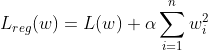
Where L(w) is the logistic loss and the hyperparameter α controls how much we want to regularize the models. In the above equation if we change the loss function to Mean Square Error(MSE), then we get Ridge Regression.
Similarly the L1 Regularized Logistic Regression looks like the following:
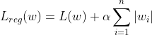
Here too if we replace the Loss function to MSE, we get Lasso Regression.
Logistic regression Assumptions :
- Binary logistic regression requires the dependent variable to be binary and Softmax regression requires the dependent variable to be ordinal.
- Observations should be independent of each other. In other words, the observations should not come from repeated measurements or matched data.
- Little or no multicollinearity among the independent variables. This means that the independent variables should not be too highly correlated with each other.
- Logistic regression assumes linearity of independent variables and log odds. although this analysis does not require the dependent and independent variables to be related linearly, it requires that the independent variables are linearly related to the log odds.
- Logistic regression typically requires a large sample size.
Now let us implement Logistic Regression using mini-batch Gradient descent and it’s variations which I have discussed in my post on Linear Regression, Refer this.
Let’s create a random set of examples:
X = np.random.rand(1000,2)
y = 2 * X[:, 0] + -3 * X[:, 1]  # True Weights = [2,-3]
y = np.round(1/(1 + np.exp(-y)))
Let’s plot this data:
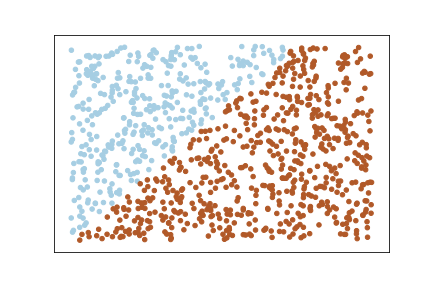
You can clearly that the data is linearly separable because we created the dataset in such a way that y is a linear combination of x. This is just for a demo purpose, in real world the dataset will not be like this.
Now let’s define a function a function that will return the probability scores:
def get_probs(X, w):
    prob = 1/(1+(np.exp(-np.dot(X,w))))
    return np.array(prob)
Now Let’s define the cross entropy Loss function:
def log_loss(X,w,y):
    a = y * np.log(get_probs(X,w))
    b = (1-y) * (np.log(1-get_probs(X,w)))
    loss = -np.sum(a+b)/X.shape[0]
    return loss
Let’s define a function that computes the Gradients of the loss function:
def get_grads(X,w,y):
    grad = np.dot((get_probs(X,w)-y),X)/X.shape[0]
    return grad
Mini-batch SGD:
w = np.array([1,-3]) #Initial Weights
eta= 0.1 # learning rate
n_iter = 4000 # Number of Iterations
batch_size = 128 #Batch size

loss = np.zeros(n_iter) #List to store the loss at each iteration

es = 0.1 #For early stopping

for i in range(n_iter):
    ind = np.random.choice(X.shape[0], batch_size)# Random indices
    loss[i] = log_loss(X[ind, :], w, y[ind])
    w = w - eta * get_grads(X[ind, :], w, y[ind])

    if(loss[i]<es): #If loss less than es we break(Early stopping)
        break
Here I’am storing the loss at each iteration in a list, so that later it can be used to plot the loss. I haven’t incorporated that here but in the full implementation present in my Github, I have incorporated those.
mini-batch SGD with Momentum:
w = np.array([1,-3]) #Initial Weights

eta = 0.05 # learning rate
alpha = 0.9 # momentum

h = np.zeros_like(w)  #This is the additional vector

es = 0.1 #For early stopping

n_iter = 4000 # Number Of iterations
batch_size = 128 #Batch Size
loss = np.zeros(n_iter) #List to store Loss at each iteration

for i in range(n_iter):
    ind = np.random.choice(X.shape[0], batch_size) # Random Indices
    loss[i] = log_loss(X[ind, :], w, y[ind])
    h = alpha * h + eta * get_grads(X[ind, :], w, y[ind]) # Update h
    w = w-h

    if(loss[i]<es): #If loss less than 'es' break(Early stopping)
        break
mini-batch SGD With Nestrov accelerated momentum:
w = np.array([1,-3]) #Initial Weights

eta = 0.05 # Learning rate
alpha = 0.9 # Momentum

h = np.zeros_like(w)  #This is the additional vector

es = 0.1 #For early stopping

n_iter = 4000 #Number of Iterations
batch_size = 128 #Batch Size
loss = np.zeros(n_iter) #List to store Loss at each iteration

for i in range(n_iter):
    ind = np.random.choice(X.shape[0], batch_size)
    loss[i] = log_loss(X[ind, :], w, y[ind])
    h = alpha * h + eta * get_grads(X[ind, :], w-alpha * h, y[ind])
    w = w-h

    if(loss[i]<es): #If loss less than 'es' break(Early stopping)
        break
RMSProp :
w = np.array([1,-3]) #Initial Weights

eta = 0.05 # learning rate
alpha = 0.9 # momentum
gt = None
eps = 1e-8
es = 0.1 #For early stopping

n_iter = 4000 #Number of Iterations
batch_size = 128 #Batch Size
loss = np.zeros(n_iter) #List to store Loss at each iteration

for i in range(n_iter):
    ind = np.random.choice(X.shape[0], batch_size) #Random Indices
    loss[i] = log_loss(X[ind, :], w, y[ind])

    gt = get_grads(X[ind, :], w, y[ind])**2
    gt = alpha*gt +(1-alpha)*gt

    w = w-(eta*get_grads(X[ind, :], w, y[ind]))/np.sqrt(gt+eps)

    if(loss[i]<es): #If loss less than 'es' break(Early stopping)
        break
Adam :
w = np.array([1,-3]) #Initial Weights

eta = 0.05 # learning rate
alpha = 0.9 # momentum
gt = None
vt = 0
beta = 0.0005

eps = 1e-8
es = 0.1 #For early stopping

n_iter = 4000 #Number of Iterations
batch_size = 128 #Batch Size
loss = np.zeros(n_iter) #List to store all the loss

for i in range(n_iter):
    ind = np.random.choice(X.shape[0], batch_size)
    loss[i] = log_loss(X[ind, :], w, y[ind])

    gt = get_grads(X[ind, :], w, y[ind])**2

    vt = (beta*vt) + (1-beta)*gt

    w = w-(eta*get_grads(X[ind, :], w, y[ind]))/np.sqrt(vt)+eps

    if(loss[i]<es):
        break
You can find the full implementation with plots in my Github account here. You can try with different values for each of these parameters and understand what changes these parameters have on the performance of the model. Here I have gone for only 2 features just for the simplicity.
References :
- https://www.oreilly.com/library/view/hands-on-machine-learning/9781491962282/
- https://en.wikipedia.org/wiki/Logistic_regression