Sequential Minimal Optimization for Support Vector Machines

In this post, I will discuss about the Sequential Minimal Optimization(SMO) which is an Optimization technique that is used for training Kernel SVM’s

In this post, I will discuss the Sequential Minimal Optimization(SMO) which is an Optimization technique that is used for training Support Vector Machines(SVM). Before getting into the discussion on SMO, I will discuss some basic Mathematics required to understand the Algorithm. Here I will start with the discussion on Lagrange Duality, Dual Form of SVM and then solving the dual form using the SMO algorithm.

Lagrange Duality

Consider the following Primal Optimization Problem :

To solve this, let us define the Lagrangian as :

Here the αi’s and βi’s are the Lagrange Multipliers. Now let us define the primal Lagrangian function as :

For any given w, if w violates any of the Primal constraints, then it can be shown that :

Now if the constraints are satisfied for a particular value of w, then p(w)=f(w). This can be summarised as follows :

Now let’s consider the minimization problem :

We have already seen that p(w) takes the same value as the objective for all values of w that satisfies the primal constraints and ∞ otherwise. So we can clearly see from the minimization problem that the solutions to this problem is same as the original Primal Problem. Now let us define the optimal value of the objective to be :

Now let us define the Dual Lagrangian function as :

Now we can pose the Dual Optimization problem as :

Now let’s define the optimal value of the dual problem objective as :

Now it can be shown that :

“Max-min” of a function will always be less than or equal to “Min-max”. Also under certain conditions, d∗=p∗. These conditions are :

This means that we can solve the dual problem instead of the primal problem. So there must exist w∗, α∗, β∗ so that w∗ is the solution to the primal and α∗ and β∗ are the solutions to the Dual Problem and p∗=d∗. Here w∗, α∗, β∗ satisfy the Karush-Kuhn-Tucker(KKT) constraints which are as follows :

Stationarity conditions :

Complimentary slackness condition :

Primal feasibility condition :

Dual feasibility condition :

Optimal Margin Classifiers :

The Primal Optimization problem for an Optimal margin Classifier is given as :

Now let us construct the Lagrangian for the Optimization problem as :

To find the dual form of the problem, we need to first minimize L(w,b,α) wrt. b and w, this can be done by setting the derivatives of L wrt. w and b to zero. So we can write this as :

For derivatives of L wrt. b, we get :

Now we can write the Lagrangian as :

But we have already seen that the last term of the above equation is zero. So rewriting the equation, so we get :

The above equation is obtained by minimizing L wrt. b and w. Now putting all this together with all the constraints, we obtain the following :

Now once we have found the optimal αi’s we can find optimal w using the following :

Having found w∗, now we can find the intercept term (b) using the following :

Now once we have fit the model’s parameters to the training set, we can get the predictions from the model for a new datapoint x using :

The model will output 1 when this is strictly greater than 0, we can also express this using the following :

Sequential Minimal Optimization

Sequential Minimal optimization (SMO) is an iterative algorithm for solving the Quadratic Programming(QP.) problem that arises during the training of Support Vector Machines(SVM). SMO is very fast and can quickly solve the SVM QP without using any QP optimization steps at all. Consider a binary classification with a dataset (x1,y1),…..,(xn,yn) where xi is the input vector and yi∈{−1,+1} which is a binary label corresponding to each xi. An optimal margin SVM is found by solving a QP. problem that is expressed in the dual form as follows :

Here C is SVM hyperparameter that controls the tradeoff between maximum margin and loss and K(xi,xj) is the Kernel Function. αi is Lagrange Multipliers. SMO is an iterative algorithm and in each step, it chooses two Lagrange Multipliers to jointly optimize and then finds the optimal values for these multipliers and updates the SVM to reflect the new optimal values. The main advantage of SMO lies in the fact that solving for two Lagrange multipliers can be done analytically even though there are more optimization sub-problems that are being solved, each of these sub-problems can be solved fast and hence the overall QP problem is solved quickly. The algorithm can be summarised using the following:

Repeat till convergence :  
{
	1. Select some pair αi and αj  
	2. Reoptimize W(α) wrt. αi and αj while holding all other αk’s fixed.
}

There are two components to SMO: An analytical solution for solving for two Lagrange Multipliers and a heuristic for choosing which multipliers to optimize.

Solving for two Lagrange Multipliers :

SMO first computes the constraints on the two multipliers and then solves for constrained minimum. Since there is a bounding constraint 0≤αi≤C on the Lagrange multipliers, these Lagrange multipliers will lie within a box. The following causes the Lagrange multipliers to lie on the diagonal :

If SMO optimized only one multiplier, it could not fulfill the above equality constraint at every step. Thus the Constrained minimum of the objective function must lie on a diagonal line segment. Therefore, one step of SMO must find an optimum of the objective function on a diagonal line segment. This can be seen from the following diagram :

Source

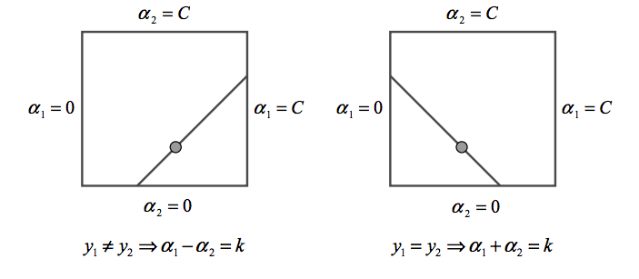
Because there are only two multipliers, the constraints can be easily displayed in two dimensions as seen above. The algorithm first computes the second Lagrange multiplier α2 and then computes the ends of the diagonal line segment in terms of α2.

If y1≠y2, then the following bounds apply to α2 :

If y1=y2, then the following bounds apply to α2 :

The second derivative of the Objective function along the diagonal is expressed as :

Under normal circumstances, η will be greater than zero and there will be a minimum along the direction of the linear equality constraint. In this case, SMO computes the minimum along the direction of the constraint :

Where :

μi is the output of the SVM for the i’th training example. The constrained minimum is found by clipping the unconstrained minimum to the ends of the line segment :

The value of α1 is computed from the new clipped α2 using:

Under normal circumstances η>0. A negative η occurs if the kernel K does not obey Mercer’s Conditions which states that for any Kernel(K), to be a valid kernel, then for any input vector x, the corresponding Kernel Matrix must be symmetric positive semi-definite. η=0 when more than one training example has the same input vector x. SMO will work even when η is not positive, in which case the objective function(ψ) should be evaluated at each end of the line segment :

SMO will move the Lagrange multipliers to the point that has the lowest value of the Objective Function. If Objective function is the same at both ends and Kernel obeys Mercer’s conditions, then the joint minimization cannot make progress, in such situations we follow the Heuristic approach, which is given below.

Heuristic for choosing which multipliers to Optimize :

According to Osuna’s Theorum, a large QP. The problem can be broken down into a series of smaller QP sub-problems. A sequence of QP. subproblems that add at least one violator to the Karush-Kuhn-Tucker(KKT) conditions is guaranteed to converge. So SMO optimizes and alters two lagrange multipliers at each step and at least one of the Lagrange multipliers violates the KKT conditions before the next step, then each step will decrease the objective function and thus by the above theorem making sure that convergence does happen.

There are two separate heuristics: one for choosing the first Lagrange multiplier and one for the second. The choice for the first heuristic forms the outer loop of SMO. The outer loop iterates over the entire training set, and determines if each example violates the KKT conditions and if it does, then it is eligible for optimization.

After one pass through the entire dataset, the outer loop of SMO makes repeated passes over the non-bound examples(examples whose Lagrange Multipliers are neither 0 nor C) until all of the non-bound examples obey the KKT conditions within ϵ. Typically ϵ is chosen to be 10^(−3).

As SMO progresses, the examples that are at the bounds are likely to stay at the bounds while the examples that are not at the bounds will move as other examples are optimized. And then finally SMO will scan the entire data set to search for any bound examples that have become KKT violated due to optimizing the non-bound subset.

Once the first Lagrange multiplier is chosen, SMO chooses the second Lagrange multiplier to maximize the size of the step taken during the joint optimization. Evaluating the Kernel Function K is time consuming, so SMO approximates the step size by the absolute value of |E1−E2|.

If E1 is positive, then SMO chooses an example with minimum error E2.
If E1 is negative, SMO chooses an example with maximum error E2.

If two training examples share an identical input vector(x), then a positive progress cannot be made because the objective function becomes semi-definite. In this case, SMO uses a hierarchy of second choice heuristics until it finds a pair of Lagrange multipliers that can make a positive progress. The hierarchy of second choice heuristics is as follows :

SMO starts iterating through the non-bound examples, searching for a second example that can make a positive progress.
If none of the non-bound examples makes a positive progress, then SMO starts iterating through the entire training set until an example is found that makes positive progress.

Both the iteration through the non-bound examples and the iteration through entire training set are started at random locations so as to not bias SMO. In situations when none of the examples will make an adequate second example, then the first example is skipped and SMO continues with another chosen first example. However, this situation is very rare.

Computing the threshold :

After optimizing αi and αj, we select the threshold b such that the KKT conditions are satisfied for the ith and jth examples. When the new α1 is not at the bounds, then the output of SVM is forced to be y1 when the input is x1, hence the following threshold(b1) is valid :

When the new α2 is not at the bounds, then the output of SVM is forced to be y2 when the input is x2, hence the following threshold(b2) is valid :

When both b1 and b2 are valid, they are equal. When both new Lagrange multipliers are at bound and if L is not equal to H, then all the thresholds between the interval b1 and b2 satisfy the KKT conditions. SMO chooses the threshold to be halfway in between b1 and b2. The complete equation for b is given as :

Now to compute Linear SVM, only a single weight vector(w) need to be stored rather than all of the training examples that correspond to non-zero Lagrange multipliers. If the joint optimization succeeds, then the stored weight vector needs to be updated to reflect the new Lagrange multiplier values. The updation step is given by :

The pseudocode for SMO is available here.