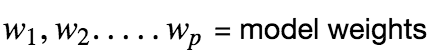
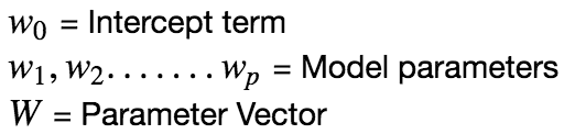
Linear Regression & Gradient Descent
In this Post, I will discuss about Linear Regression and Gradient Descent along with their implementation in Python.
 on [Unsplash](https://unsplash.com?utm_source=medium&utm_medium=referral)](https://cdn-images-1.medium.com/max/10368/0*O5R1cW3XdAn6KWW6)
Introduction:
Linear Regression attempts to model the relationship between two variables by fitting a linear equation to the observed data. One variable is considered to be an explanatory variable(independent variable x) and other is considered to be a dependent variable(y). But first, we must understand if there is a relationship between the variables of interest: this does not necessarily mean one causes another but there is some significant association between the two variables. A scatterplot can be used to determine the strength of the relationship between the two variables. If there is no relationship between the exploratory and dependent variable, then there is no point in fitting a linear model.A valuable numerical association between two variables is the correlation coefficient which is a value between [-1,1] indicating the strength of association of the observed data for two variables. A linear regression line has an equation of the form:
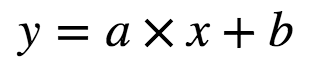
Here x is the independent or exploratory variable and y is the dependent variable, a is the intercept while b is the slope of the line.
Let’s say our Dataset Xis given as:
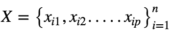
Where n is the number of features.
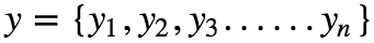
Let the dependent variable be y, given as :
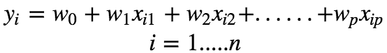
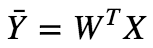
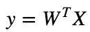
Assuming that there is a linear dependency between x and y, the model prediction can be given as :
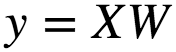
Using vector notation, we can write this as :
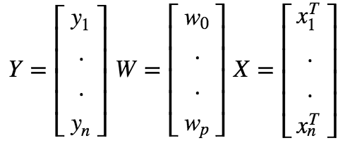
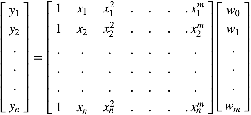
Now we can express the prediction matrix as :
Linear Regression Assumptions :
-
Linearity: The relationship between X and Y must be linear. We can check this using Scatter Plots.
-
Normality: For any value of X and Y, it should be normally distributed. We can check this using (Q-Q) plot. Normality can be checked with a goodness of fit test(K-S) test. When data is not normally distributed, we can use non-linear transformation(eg: log-transformation) to solve the issue.
-
Homoscedasticity: This is a situation in which the random disturbance in the relationship between the independent variables and the dependent variable or noise is the same across all values of the independent variables.
-
No or Little Multicollinearity: Multicollinearity happens when independent variables are too highly correlated with each other.
Test For Multicollinearity :
1.Correlation Matrix: Compute Pearson’s Bivariate Correlation among all independent variables and correlation coefficient must be smaller than 1.
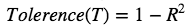
2.Tolerence: Measures the influence of one independent variable on all the independent variables.
-
Regress each independent variable on all other independent value.
-
Subtract each R² value from 1.
-
If T<1 => Might be multicollinearity.
-
If T<0.01 => Multicollinearity.
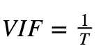
3.Variance Inflation Factor :
-
If VIF = 1, No multicollinearity.
-
If VIF = Between 1 and 5, then moderately correlated.
-
If VIF > 5, then there is high correlation.
Mean Centering could help solve the problem of Multicollinearity. Also remove independent variables with high VIF values.
Training Linear Regression :
We need to measure the goodness of fit or how well the model fits the data.
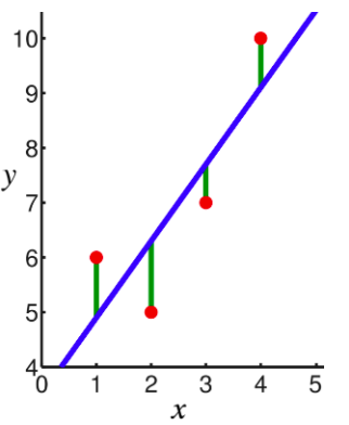
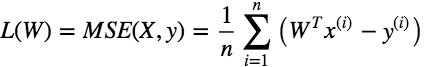
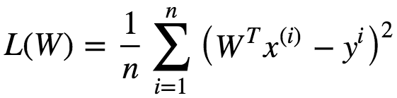
In linear regression, the observations (red) are assumed to be the result of random deviations (green) from an underlying relationship (blue) between a dependent variable (y) and an independent variable (x). In Linear Regression we try to minimize the deviations. How to measure this deviation. One Common metric for that is the Mean(Mean Square Error). The predictions(y) can be given as following:
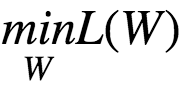
To train a Linear Regression model, we need to find the value of W that minimizes the MSE.
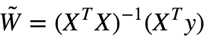
There is a closed form equation to find the W that minimizes this loss/cost function also called Normal Equation which is given as:
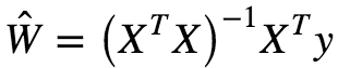
For the derivation of the above closed form equation click here
Ŵ is the value of W that minimizes the loss function. y = Vector of target values containing {y ¹….yᵐ} . However computing the inverse of for an n×n matrix is about O(n³) depending on the implementation. Hence this is a very slow process. However for extremely large datasets that might not fit into RAM, this method cannot be applied. But Predictions are extremely fast≈O(m) where m = number of features.
Gradient Descent
This is a generic optimization technique capable of finding optimal solutions to a wide range of problems. Thee General idea is to tweak the parameters iteratively to minimize a cost function. For a GD to work, the loss function must be differentiable. This method is also called the steepest descent method.
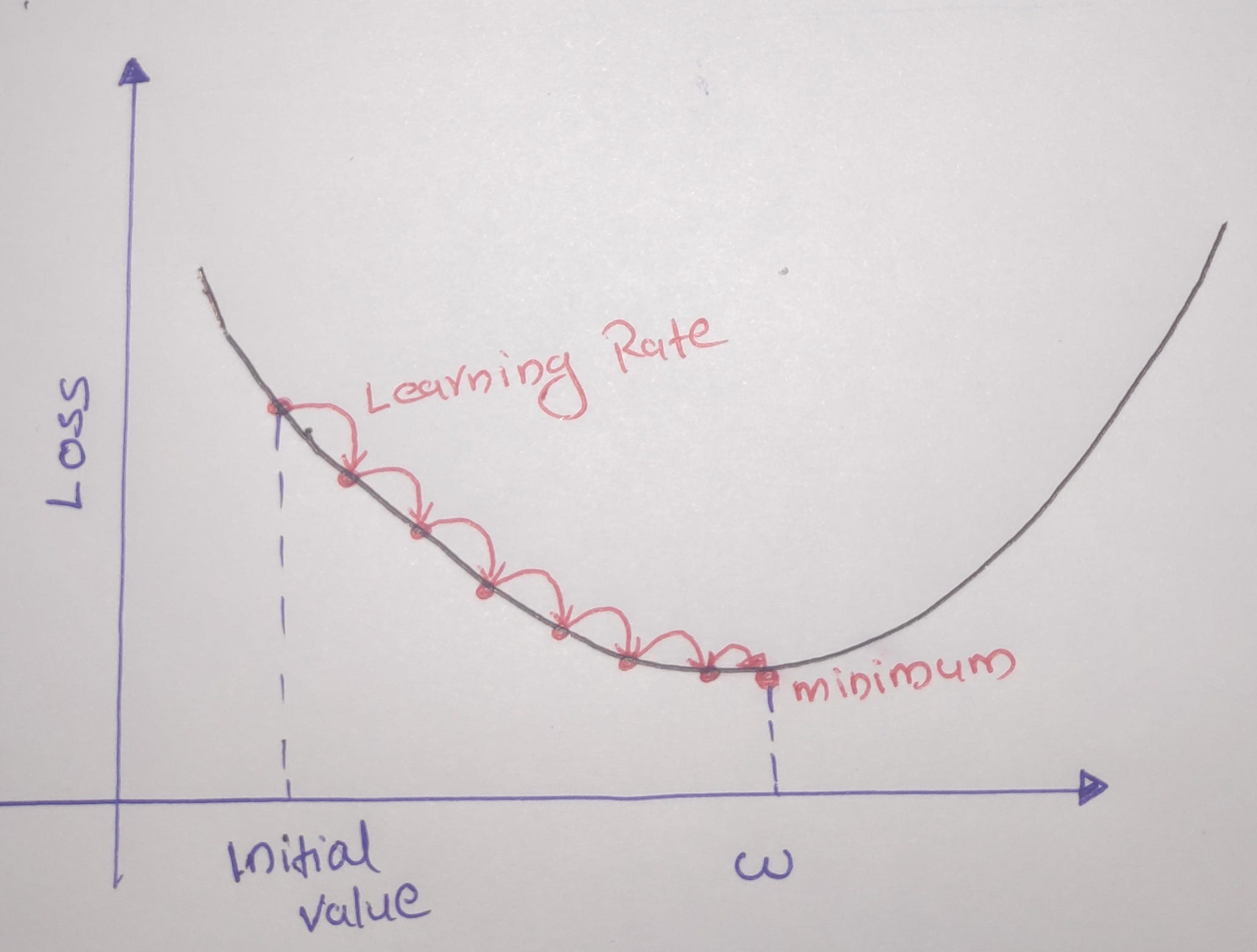 Image by Author
-
If Learning Rate = too small => Takes too much time to converge.
-
If Learning Rate = Large => May not converge as it misses the minimum.
Gradient Descent works well when there are convex functions. What if the functions are not convex like the below figure :
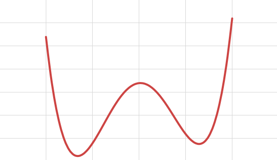
Here depending on the initial starting point, the Gradient Descent may end up stuck in local minima. In this case we can reset the initial value and do gradient descent again. However the Loss function for Linear Regression(MSE) is a convex function ie if we pick any two points in the curve, the line segment joining them never crosses the line. This means that there are no local minima but a single global minimum and also it is a continuous function. Gradient Descent is guaranteed to approach arbitrarily close to the global minimum. Training a model means searching for a combination of model parameters that minimizes the Loss function.
We need to find a direction where function decreases and we need to take a step in this direction.
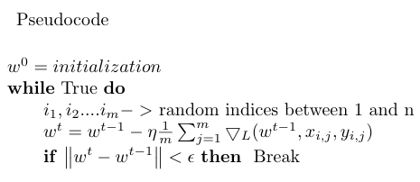
Optimization Problem:
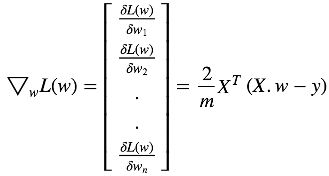
Let the initial weights be w⁰. The gradient vector is given by :
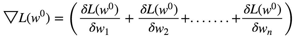
This Gradient Vector points in the direction of Steepest Ascent at **w⁰. **This function has a fast decreasing rate in the direction of negative gradient.
In matrix Notation we can write this as :
Gradient Descent Step :
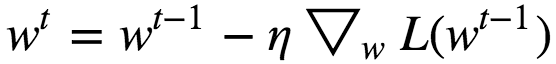
Where 𝜂 = Learning Rate
When 𝜂 = too small => The Algorithm eventually reach the optimal solution, but it will take too much time.
When 𝜂 = too large => The Algorithm diverges jumping all over the place and actually getting further and further away from the solution at every step.
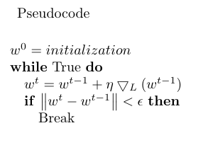
We can use GridSearch to find a good Learning Rate. We can set the number of iterations to be large but to interrupt the algorithm when the gradient vector becomes tiny, we can calculate the norm of the Gradient vector at every step and if it is less than a tiny value (ϵ), Gradient Descent has reached minimum so we must halt the Gradient Descent. Gradient Descent works even in spaces of any number of dimensions even in infinite dimension ones.
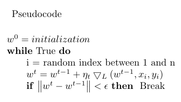
Stochastic Gradient Descent
Batch Gradient Descent or Gradient Descent requires the whole training set in memory to compute the gradients at every step. This makes it slow when train set is huge. Also if the training dataset doesn’t fit the memory we might not be able to use Gradient Descent. In Stochastic Gradient Descent(SGD), we just pick a random instance in the training set at each step and then compute the gradients based only on that single instance. This makes the algorithm fast since it has very little data to manipulate at every iteration. It also makes possible to train huge datasets that does not fit into memory. Due to it’s Stochastic(random) nature, the algorithm is much less regular than G.D. instead of decreasing till it reaches the minimum, the Loss function will bounce up and down, decreasing only on average ie it leads to Noisy updates. Over the time it will end up closer to minimum, but once it gets there it will continue to bounce around, never settling down. Once Algorithm stops final parameters are good but not optimal. Each step is a lot faster to compute for SGD than for GD, as it uses only one training example. One advantage of having such updates is that, when there is an irregular function, then this can help the algorithm jump out of local minima, So SGD has better chance of finding global minimum than Gradient Descent.
This Randomness can help to avoid local minima, but what if the algorithm never settle at a minimum? The following are some of the hacks that could be used to avoid such a situation:
-
Gradually reduce the learning rate. The algorithm starts with large Learning Rate and then slowly reduce the learning rate and it becomes smaller and smaller allowing the algorithm to settle at Global minimum. This is called simulated annealing.
-
The function that determines the Learning Rate at each iteration is called learning rate scheduler.
However the following cases must be taken care of :
-
If Learning Rate is reduced too quickly, then the algorithm may get stuck in Local minima or Frozen halfway.
-
If Learning Rate is reduced too slowly, then we might jump around the minimum for a long time and end up in suboptimal solution.
Mini-Batch Stochastic Gradient Descent
Here, instead of computing gradients based on full training set (or) just a single instance, mini-batch GD computes the gradients on small random sets of instances called mini-batches. The main advantage of mini-batch SGD over SGD is that we can get performance boost from hardware optimization of matrix operations especially with a GPU. Both Mini-Batch SGD as well as SGD tends to walk around minimum but GD will converge to minimum, however GD takes more time to take each step. Both SGD and mini-batch SGD would also reach minimum if good learning rate is chosen.
The difference between Gradient Descent, Mini-Batch Gradient Descent and Stochastic Gradient Descent is the number of examples used to perform a single updation step.
Polynomial Regression
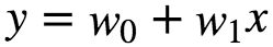
What if the data is more complex than simple straight line and cannot be fit with simple Linear Regression. Polynomial Regression is a regression analysis in which the relationship between an independent variable(X) and dependent variable(y) is modelled as an n th degree polynomial in X. Fits a non-linear relationship between the value x and corresponding conditional mean of y denoted as : E(y|x). Although polynomial regression fits a non-linear model to the data, as a statistical estimation problem, it is linear, in the sense that the regression function E(y|x) is linear in the unknown parameters that are estimated from the data. Polynomial regression is considered as special case of multiple linear regression. The goal of Polynomial Regression is to model the expected value of dependent variable y in terms of independent variable(or vector of independent variables) x. The model prediction for a simple Linear Regression is given as :
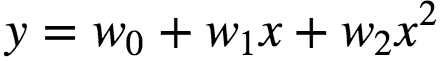
In many settings, such a linear relationship may not hold. A quadratic model of the form will be like:
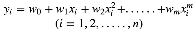
In general, we can model an expected value of y as an nth degree polynomial, yielding the general polynomial regression model:

The models are all linear from the point of view of estimation, since the regression function is linear in terms of the unknown parameters w0,…,wn.
So for Least Squares analysis, the computational and Inferential problem of polynomial regression can be completely addressed using the techniques of multiple regression. This is done by treating x, x²….. as being distinct independent variables in a multiple regression model.
Matrix form and Calculation of estimates
This can be expressed in matrix notation as :
In pure Matrix Notation, this can be expressed as :
The closed form solution for the this is given as :
We can solve this using Gradient Descent as well.
Regularized Linear Models
Overfitting :
This occurs when a statisticsl model/ ML algorithm captures the noise of the data or intuitively it happens when model (or) algorithm fits data too well. Specifically Overfitting Occurs if the model (or) Algorithm shows low bias but high Variance. Overfitting models perform well on training data but generalizes poorly according to Cross-Validation metrics.
How to prevent it :
-
Cross-Validation
-
Train with more data
-
Feature Selection
-
Early Stopping
-
Regularization
-
Ensembling
Underfitting :
This occurs when a statistical model/ML algorithm cannot capture the underlying trend in the data or intuitively it happens when the model/Algorithm does not fit the data well enough. Specifically, underfitting occurs if model (or) Algorithm shows low variance but high bias. This is a result of excessively simple model. Underfitted models perform poorly in both train and validation data set.
How to prevent it :
-
Increase the number of Parameters in ML models
-
Increase complexity of the model
-
Increasing the training time untill cost function in ML model is minimized.
Generalization Error :
Generalization error can be classified into 3 types. They are :
-
Bias : This is due to wrong assumptions such as like data is linear when it is actually quadratic. When a model has high bias then it indicates that the model is an underfit model.
-
Variance : This is due to model’s excessive sensitivity to small variations in the training data. A model with high degrees of freedom(higher degree polynomial) is likely to have high variance and thus overfit the training data.
-
Irreducible Error : This is due to noisiness in the data, this can be reduced by cleaning the data properly.
Bias-Variance tradeoff :
Increase in model’s complexity will typically increase it’s Variance and reduce it’s bias. Reducing a model’s complexity will typically increase it’s bias and reduce it’s variance. This is why it is called as Bias-Variance Tradeoff.
Ridge Regression :
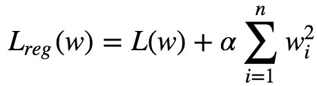
A good way to reduce overfitting is to regularize the model. The fewer degrees of freedom it has the harder it will be for the model to overfit the data. eg: A simple way to regularize a polynomial model is to reduce the number of polynomial degrees. Ridge regression is a regularized version of Linear Regression with regularization term added to it. The regularization term is given as :
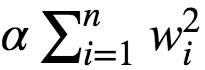
This forces the Learning Algorithm to not only fit the data, but also keep the model weights as small as possible. Regularization term must be added to the loss function only during training. Once the model is trained, we evaluate the model using unregularized performance measure. The hyperparameter α controls how much we want to regularize the models:
-
If α = 0, Then Ridge Regression becomes Linear Regression.
-
If α = V.large, then all weights end up close to zero and results in a flat line going through the mean of data.
Here the bias term w⁰ is not regularized.
If w is the weight vector, then the regularization term is simply equal L2 norm of the weight vector. There exists a closed-form solution to Ridge regression, which is given as :
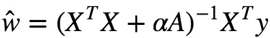
Where A is an n×n identity matrix except with 0 in top-left which corresponds to the bias term.
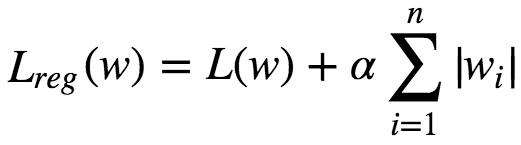
Lasso Regression :
Lasso(Least Absolute Shrinkage & Selection Operator Regression) is a Regularized version of Linear Regression. Adds a regularization term to the Loss function. It uses L1 norm of weight vector instead of L2 norm.
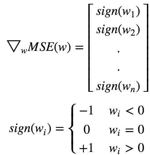
An important characteristic of L1 regularization is that it completely eliminates the weights of least importance(ie set them to 0). Lasso Regression automatically performs feature selection and outputs a sparse model.Lasso function is not differentiable at wi **= 0(for i=1,2,3…n). But GD. still works fine if we use a subgradient vector instead when any **wi=0.
Elastic Net :
It is in between Ridge and Lasso Regression. The regularization term is a simple mix of both Ridge and Lasso Regression terms and we can control it with the mix ratio(r).
-
If r=0 = > E.N ≈Ridge Regression
-
If r=1 = > E.N ≈Lasso Regression
when do we choose Elastic Net over plain L.R :
-
It is always preferable to have atleast a bit of regularization, so generally you should avoid plain LR.
-
Ridge is good, but if we need to apply feature selection also, then go for Lasso or EN. since they tend to reduce the weights of useless features down to zero.
-
Elastic Net is preferred over Lasso since Lasso may behave erratically when the number of Features is greater than the number of training instances (or) when several features are strongly correlated.
Extentions to Gradient Descent
Momentum Approach
Stochastic gradient descent with momentum remembers the update Δw at each iteration, and determines the next update as a linear combination of the gradient and the previous update. Here an additional vector (h) is maintained at every iteration.
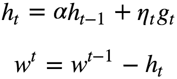
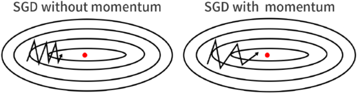
ht = Weighted sum of gradients from all the previous iteration and from this iteration also. Tends to move in the same direction as of previous steps. ht cancels some coordinates that lead to oscillation of gradients and help to achieve better convergence. ie the momentum term increases for dimensions whose gradients point in the same directions and reduces updates for dimensions whose gradients change directions. As a result, we gain faster convergence and reduced oscillation. when using momentum, imagine that we push a ball down a hill. The ball accumulates momentum as it rolls downhill, becoming faster and faster on the way (until it reaches its terminal velocity if there is air resistance, i.e. α<1. ht accumulates values along dimensions where the gradients have same sign. Usually α = 0.9.
Nestrov Accelerated Momentum
A ball that rolls down a hill, blindly following the slope, is highly unsatisfactory. We’d like to have a smarter ball, a ball that has a notion of where it is going so that it knows to slow down before the hill slopes up again.
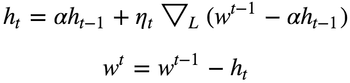
Here we first step in the direction of ht to get some new approximation of parameter vector and then calculate gradient at the new point. And then move in the negative of that gradient vector this can be clearly seen from the above diagram. Both Nestrov Accelerated Momentum as well as Momentum approach is sensitive to learning rate(η).
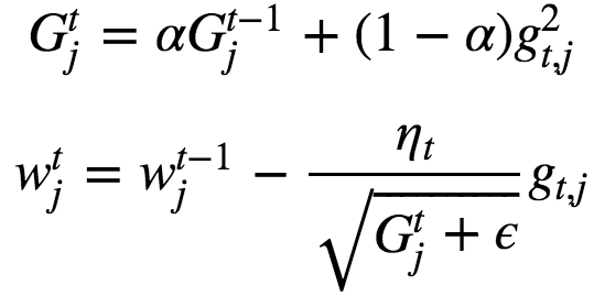
AdaGrad :
Adagrad is a modified SGD with per-parameter learning rate. This increases the learning rate for sparser parameters and decreases the learning rate for ones that are less sparse. Improves convergence performance over standard stochastic gradient descent in settings where data is sparse and sparse parameters are more informative. Examples of such applications include natural language processing and image recognition.
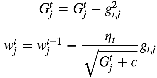
gt,j = Gradient at iteration t with respect to parameter j. Here base learning rate can be fixed : ηt = 0.01. G= Sum of squares of gradients from all previous iterations. Gtj always increases which leads to early stopping which is a bit of problem too because sometimes G becomes too large that it results in stopping before it reaches the minimum. AdaGrad can be applied to non-convex optimization problems also.
RMSProp
RMSProp (for Root Mean Square Propagation) is also a method in which the learning rate is adapted for each of the parameters. RMSprop divides the learning rate by an exponentially decaying average of squared gradients.
RMSProp has shown excellent adaptation of learning rate in different applications. RMSProp can work with mini-batches as well. Typically α = 0.9 and default value of learning rate is set to η=0.001.
Adam
Adaptive Moment Estimation(Adam) is an update to the RMSProp optimizer ie it computes the learning rates for each parameters adaptively. In addition to storing an exponentially decaying average of past squared gradients like, Adam also keeps an exponentially decaying average of past gradients, similar to momentum. Momentum can be seen as a ball running down a slope, Adam behaves like a heavy ball with friction, which thus prefers flat minima in the error surface.
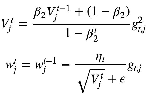
The approximation V has bias towards 0 especially at initial steps cos we initialize β2 with 0. So iorder to get rid of this bias, we divide by 1−β2t. This normalization allows to get rid of the bias.
Now let’s implement Linear Regression using some of the methods described above. Here we will use only min-batch SGD and it’s variations in python.
    #Create random set of Examples :
    X = np.random.rand(1000,4)
    y = 3 * X[:, 0] + 10 * X[:, 1] + -2 * X[:, 2] + -3 * X[:, 3]
    # True Weights = [3,10,-2,-3]
Here for simplicity we will not consider the bias(intercept) term.
Let’s define the loss function :
# Define the MSE loss function
def mse_loss(X,w,y):
pred = np.dot(X,w)
mse = (np.square(y-pred)).mean()
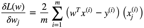
return mseLet’s define a function to compute the Gradients:
    #This will return the gradients
    def get_grads(X,w,y):
        m = X.shape[0]
        return (2/m)*np.dot(X.T,np.dot(X,w)-y)
Simple mini-batch SGD
    w = np.array([0,0,0,0]) #Initial Weights
    eta= 0.1 # learning rate

    n_iter = 1000 # Number of Iterations
    batch_size = 128 #Batch Size

    loss = np.zeros(n_iter) #List to store the loss at each iteration

    for i in range(n_iter):
        ind = np.random.choice(X.shape[0], batch_size) #random indices

        loss[i] = mse_loss(X[ind, :], w, y[ind]) #compute loss

        w = w - eta*get_grads(X[ind, :], w, y[ind]) #weight updation
Here I’am storing the loss at each iteration in a list, so that later it can be used to plot the loss as well as apply early stopping. I haven’t incorporated that here but in the full implementation present in my Github, I have incorporated those changes.
mini-batch SGD with Momentum:
    w = np.array([0,0,0,0])

    eta = 0.05 # learning rate
    alpha = 0.9 # momentum

    h = np.zeros_like(w)  #This is the additional vector

    n_iter = 1000
    batch_size = 128
    loss = np.zeros(n_iter)

    for i in range(n_iter):
        ind = np.random.choice(X.shape[0], batch_size)

        loss[i] = mse_loss(X[ind, :], w, y[ind])

        h = alpha*h + eta*get_grads(X[ind, :], w, y[ind]) #update 'h'

        w = w-h #Weight updation
mini-batch SGD With Nestrov accelerated momentum:
    w = np.array([0,0,0,0]) #Initial Weights

    eta = 0.05 # learning rate

    alpha = 0.9 # momentum

    h = np.zeros_like(w)  #This is the additional vector

    n_iter = 1000
    batch_size = 128
    loss = np.zeros(n_iter)

    for i in range(n_iter):
        ind = np.random.choice(X.shape[0], batch_size)

        loss[i] = mse_loss(X[ind, :], w, y[ind])

        h = alpha*h + eta*get_grads(X[ind, :], w-alpha*h, y[ind])

        w = w-h
As you can clearly see the the only change in nestrov accelerated momentum is in the updation of the vector h.
RMSProp :
    w = np.array([0,0,0,0]) #Initial Weights

    eta = 0.05 # learning rate
    alpha = 0.9 # momentum
    gt = None
    eps = 1e-8

    n_iter = 1000
    batch_size = 128
    loss = np.zeros(n_iter)

    for i in range(n_iter):
        ind = np.random.choice(X.shape[0], batch_size)
        loss[i] = mse_loss(X[ind, :], w, y[ind])

        gt = get_grads(X[ind, :], w, y[ind])**2
        gt = alpha*gt +(1-alpha)*gt

        w = w-(eta*get_grads(X[ind, :], w, y[ind]))/np.sqrt(gt+eps)
Adam :
    w = np.array([0,0,0,0]) #Initial Weights

    eta = 0.05 # learning rate
    alpha = 0.9 # momentum
    gt = None
    vt = 0
    beta = 0.0005
    eps = 1e-8

    n_iter = 1000
    batch_size = 128
    loss = np.zeros(n_iter)

    for i in range(n_iter):
        ind = np.random.choice(X.shape[0], batch_size)
        loss[i] = mse_loss(X[ind, :], w, y[ind])

        gt = get_grads(X[ind, :], w, y[ind])**2

        vt = (beta*vt) + (1-beta)*gt

        w = w-(eta*get_grads(X[ind, :], w, y[ind]))/np.sqrt(vt)+eps
The full implementation along with plots can be found in my Github account here.
References :
-
https://datascience-enthusiast.com/DL/Optimization_methods.html
-
https://statisticsbyjim.com/regression/multicollinearity-in-regression-analysis/
-
Sebastian Ruder (2016). An overview of gradient descent optimisation algorithms. arXiv preprint arXiv:1609.04747.