Eigendecomposition, SVD and PCA

In this post, I will discuss some basic linear algebra, Eigendecomposition, SVD and PCA.

Photo by Markus Spiske on Unsplash

In this article, I will discuss Eigendecomposition, Singular Value Decomposition(SVD) as well as Principal Component Analysis. Before going into these topics, I will start by discussing some basic Linear Algebra and then will go into these topics in detail.

Basics Of Linear Algebra :

• Scalars: A scalar is just a single number. Scalars are written in italics and in lower case. “Let s ∈ R be the slope of the line,” while defining a real-valued scalar, or “Let n ∈ N be the number of units,” while defining a natural number scalar.
• Vectors: A vector is an array of numbers arranged in specific order. We can identify each individual number by its index in that ordering. A vector could be a row vector or a column vector. Typically we give vectors lowercase names in bold typeface, such as x. By default Vectors are Column vectors unless it’s explicitly mentioned.
• Matrix: A matrix is a 2-D array of numbers, so each element is identified by two indices instead of just one. We usually give matrices uppercase variable names with bold typefaces, such as A. If a real-valued matrix A has a height of m and a width of n, then we say that A ∈ R(m×n). A(1,1)is the upper left entry of A and A(m,n)is the bottom right entry.
• Tensors: An array with more than two axes is called a Tensor.In the general case, an array of numbers arranged on a regular grid with a variable number of axes is known as a tensor. We denote a tensor named “A” with this typeface: A. We identify the element of A at coordinates. (i, j, k) by writing A(i,j,k).
• Transpose: The transpose of a matrix is the mirror image of the matrix across a diagonal line, called the main diagonal, running down and to the right, starting from its upper left corner. We denote the transpose of a matrix A as A^T and is defined as follows :

• Vectors can be thought of as matrices that contain only one column. The transpose of a vector is, therefore, a matrix with only one row.
• Addition Of Matrices: We can add matrices to each other, as long as they have the same shape, just by adding their corresponding elements which can be defined as: C = A + B. Where:

• We can also add a scalar to a matrix or multiply a matrix by a scalar, just by performing that operation on each element of a matrix: D = a·B+c where:

• We can also do the addition of a matrix and a vector, yielding another matrix: C=A+b, Where :

Here we add b to each row of the matrix. This is also called as broadcasting.

Multiplying Matrices and Vectors :

The matrix product of matrices A and B is a third matrix C. In order for this product to be defined, A must have the same number of columns as B has rows. If A is of shape m × n and B is of shape n × p, then C has a shape of m × p. We can write the matrix product just by placing two or more matrices together :

The product operation is defined by :

This is also called as the Dot Product. The following are some of the properties of Dot Product :

• Distributive property :

• Associativity :

• Dot Product is not Commutative :

Identity Matrix: An identity matrix is a matrix that does not change any vector when we multiply that vector by that matrix. All the entries along the main diagonal are 1, while all the other entries are zero.

Inverse of a Matrix: The matrix inverse of A is denoted as A^(−1), and it is defined as the matrix such that :

This can be used to solve a system of linear equations of the type Ax = b where we want to solve for x:

Linear independence and Span :

A set of vectors is linearly independent if no vector in a set of vectors is a linear combination of the other vectors. The span of a set of vectors is the set of all the points obtainable by linear combination of the original vectors.

Norms :

Used to measure the size of a vector. Formally the Lp norm is given by:

On an intuitive level, the norm of a vector x measures the distance from the origin to the point x. The L² norm, with p = 2, is known as the Euclidean norm, which is simply the Euclidean distance from the origin to the point identified by x. The L² norm is often denoted simply as ||x||,with the subscript 2 omitted. It is also common to measure the size of a vector using the squared L² norm, which can be calculated simply as :

The squared L² norm is more convenient to work with mathematically and computationally than the L² norm itself. In many contexts, the squared L² norm may be undesirable because it increases very slowly near the origin. In these cases, we turn to a function that grows at the same rate in all locations, but that retains mathematical simplicity: the L¹ norm :

The L¹ norm is commonly used in machine learning when the difference between zero and nonzero elements is very important.

Frobenius norm: Used to measure the size of a matrix. Also called Euclidean norm (also used for vector L². norm) :

It is also equal to the square root of the matrix trace of AA^(H), where A^(H) is the conjugate transpose :

Trace of a square matrix A is defined to be the sum of elements on the main diagonal of A. The trace of a matrix is the sum of its eigenvalues, and it is invariant with respect to a change of basis.

EigenValues And EigenVectors:

An eigenvector of a square matrix A is a nonzero vector v such that multiplication by A alters only the scale of v and not the direction :

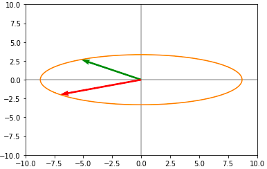
The scalar λ is known as the eigenvalue corresponding to this eigenvector. The vector Av is the vector v transformed by the matrix A. This transformed vector is a scaled version (scaled by the value λ) of the initial vector v. If v is an eigenvector of A, then so is any rescaled vector sv for s ∈ R, s != 0. Moreover, sv still has the same eigenvalue. Consider the following vector(v) :

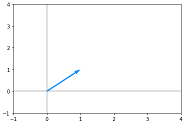
import numpy as np  
v = np.array([[1], [1]])

Let’s plot this vector and it looks like the following :

Now consider the matrix(A):

A = np.array([[5, 1], [3, 3]])

Now let’s take the dot product of A and v and plot the result, it looks like the following :

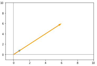
Here, the blue vector is the original vector(v) and the orange is the vector obtained by the dot product between v and A. Here we can clearly observe that the direction of both these vectors are same, however, the orange vector is just a scaled version of our original vector(v). So we can say that that v is an eigenvector of A. eigenvectors are those Vectors(v) when we apply a square matrix A on v, will lie in the same direction as that of v.

Eigendecomposition :

Suppose that a matrix A has n linearly independent eigenvectors {v1,….,vn} with corresponding eigenvalues {λ1,….,λn}. We can concatenate all the eigenvectors to form a matrix V with one eigenvector per column likewise concatenate all the eigenvalues to form a vector λ. The Eigendecomposition of A is then given by :

Decomposing a matrix into its corresponding eigenvalues and eigenvectors help to analyse properties of the matrix and it helps to understand the behaviour of that matrix. Say matrix A is real symmetric matrix, then it can be decomposed as :

where Q is an orthogonal matrix composed of eigenvectors of A, and Λ is a diagonal matrix. Any real symmetric matrix A is guaranteed to have an Eigen Decomposition, the Eigendecomposition may not be unique. If any two or more eigenvectors share the same eigenvalue, then any set of orthogonal vectors lying in their span are also eigenvectors with that eigenvalue, and we could equivalently choose a Q using those eigenvectors instead.

What does Eigendecomposition tell us?

• The matrix is singular(|A|=0) if and only if any of the eigenvalues are zero. The Eigendecomposition of a real symmetric matrix can also be used to optimize quadratic expressions of the form :

• Whenever x is equal to an eigenvector of A, f takes on the value of the corresponding eigenvalue. The maximum value of f within the constraint region is the maximum eigenvalue and its minimum value within the constraint region is the minimum eigenvalue.
• A matrix whose eigenvalues are all positive is called positive definite. A matrix whose eigenvalues are all positive or zero valued is called positive semidefinite. If all eigenvalues are negative, the matrix is negative definite. If all eigenvalues are negative or zero valued, it is negative semidefinite.
• Positive semidefinite matrices are guarantee that :

• Positive definite matrices additionally guarantee that :

Singular Value Decomposition

Singular Value Decomposition(SVD) is a way to factorize a matrix, into singular vectors and singular values. A singular matrix is a square matrix which is not invertible. Alternatively, a matrix is singular if and only if it has a determinant of 0. The singular values are the absolute values of the eigenvalues of a matrix A. SVD enables us to discover some of the same kind of information as the eigen decomposition reveals, however, the SVD is more generally applicable. Every real matrix has a singular value decomposition, but the same is not true of the eigenvalue decomposition. The singular value decomposition is similar to Eigen Decomposition except this time we will write A as a product of three matrices :

U and V are orthogonal matrices. D is a diagonal matrix (all values are 0 except the diagonal) and need not be square. The columns of U are called the left-singular vectors of A while the columns of V are the right-singular vectors of A. The values along the diagonal of D are the singular values of A. Suppose that A is an m ×n matrix, then U is defined to be an m × m matrix, D to be an m × n matrix, and V to be an n × n matrix.

The intuition behind SVD is that the matrix A can be seen as a linear transformation. This transformation can be decomposed in three sub-transformations: 1. rotation, 2. re-scaling, 3. rotation. These three steps correspond to the three matrices U, D, and V. Now let’s check if the three transformations given by the SVD are equivalent to the transformation done with the original matrix.

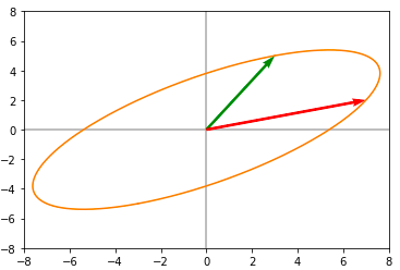
Consider a unit circle given below :

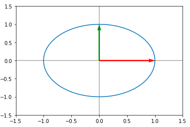
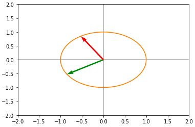
Here the red and green are the basis vectors. Not let us consider the following matrix A :

A = np.array([[3 , 7],[5, 2]])

Applying the matrix A on this unit circle, we get the following :

Now let us compute the SVD of matrix A and then apply individual transformations to the unit circle:

U, D, V = np.linalg.svd(A)

Now applying U to the unit circle we get the First Rotation :

Now applying the diagonal matrix D we obtain a scaled version on the circle :

Now applying the last rotation(V), we obtain the following :

Now we can clearly see that this is exactly same as what we obtained when applying A directly to the unit circle. Singular Values are ordered in descending order. They correspond to a new set of features (that are a linear combination of the original features) with the first feature explaining most of the variance. To find the sub-transformations :

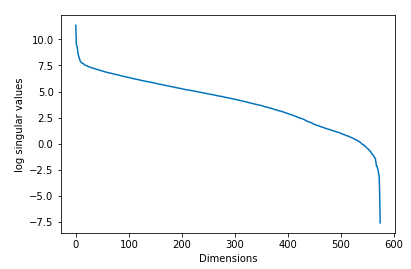
Truncated SVD :

Now we can choose to keep only the first r columns of U, r columns of V and r×r sub-matrix of D ie instead of taking all the singular values, and their corresponding left and right singular vectors, we only take the r largest singular values and their corresponding vectors. We form an approximation to A by truncating, hence this is called as Truncated SVD. How to choose r? If we choose a higher r, we get a closer approximation to A. On the other hand, choosing a smaller r will result in loss of more information. So we need to choose the value of r in such a way that we can preserve more information in A. One way pick the value of r is to plot the log of the singular values(diagonal values σ) and number of components and we will expect to see an elbow in the graph and use that to pick the value for r. This is shown in the following diagram :

However, this does not work unless we get a clear drop-off in the singular values. In real-world we don’t obtain plots like the above. Most of the time when we plot the log of singular values against the number of components, we obtain a plot similar to the following :

What do we do in case of the above situation? We can use the ideas from the paper by Gavish and Donoho on optimal hard thresholding for singular values. Their entire premise is that our data matrix A can be expressed as a sum of two low rank data signals :

Here the fundamental assumption is that :

That is noise has a Normal distribution with mean 0 and variance 1. If Data has low rank structure(ie we use a cost function to measure the fit between the given data and its approximation) and a Gaussian Noise added to it, We find the first singular value which is larger than the largest singular value of the noise matrix and we keep all those values and truncate the rest.

Case 1(Best Case Scenario) :

A is a Square Matrix and γ is known. Here we truncate all σ<τ(Threshold). The Threshold τ can be found using the following :

Case 2:

A is a Non-square Matrix (m≠n) where m and n are dimensions of the matrix and γ is not known, in this case the threshold is calculated as:

β is the aspect ratio of the data matrix β=m/n, and :

Principal Components Analysis (PCA)

Suppose we have ‘m’ data points :

and we wish to apply a lossy compression to these points so that we can store these points in a lesser memory but may lose some precision. So the objective is to lose as little as precision as possible. So we convert these points to a lower dimensional version such that:

If ‘l’ is less than n, then it requires less space for storage. We need to find an encoding function that will produce the encoded form of the input f(x)=c and a decoding function that will produce the reconstructed input given the encoded form x≈g(f(x)). The encoding function f(x) transforms x into c and the decoding function transforms back c into an approximation of x.

Constraints :

• The decoding function has to be a simple matrix multiplication: g(c)=Dc. When we apply the matrix D to the Dataset of new coordinate system, we should get back the dataset in the initial coordinate system.
• The columns of D must be orthogonal(D is semi-orthogonal D will be an Orthogonal matrix when ’n’ = ‘l’).
• The columns of D must have unit norm.

Finding the encoding function :

We know g(c)=Dc. We will find the encoding function from the decoding function. We want to minimize the error between the decoded data point and the actual data point. That is we want to reduce the distance between x and g(c). We can measure this distance using the L² Norm. We need to minimize the following:

We will use the Squared L² norm because both are minimized using the same value for c. Let c∗ be the optimal c. Mathematically we can write it as :

But Squared L² norm can be expressed as :

Applying this here, we get :

By the distributive property, we get:

Now by applying the commutative property we know that :

Applying this property we now get :

The first term does not depend on c and since we want to minimize the function according to c we can just ignore this term :

Now by Orthogonality and unit norm constraints on D :

Now we can minimize this function using Gradient Descent. The main idea is that the sign of the derivative of the function at a specific value of x tells you if you need to increase or decrease x to reach the minimum. When the slope is near 0, the minimum should have been reached.

We want c to be a column vector of shape (l, 1), so we need to take the transpose to get :

To encode a vector, we apply the encoder function :

Now the reconstruction function is given as :

Choosing the encoding matrix D

Purpose of the PCA is to change the coordinate system in order to maximize the variance along the first dimensions of the projected space. Maximizing the variance corresponds to minimizing the error of the reconstruction. Since we will use the same matrix D to decode all the points, we can no longer consider the points in isolation. Instead, we must minimize the Frobenius norm of the matrix of errors computed over all dimensions and all points :

We will start to find only the first principal component (PC). For that reason, we will have l = 1. So the matrix D will have the shape (n×1). Since it is a column vector, we can call it d. Simplifying D into d, we get :

Where r(x) is given as :

Now plugging r(x) into the above equation, we get :

We need the Transpose of x^(i) in our expression of d*, so by taking the transpose we get :

Now let us define a single matrix X, which is defined by stacking all the vectors describing the points such that :

We can now rewrite the problem as :

We can simplify the Frobenius norm portion using the Trace operator :

Now using this in our equation for d*, we get :

Now Tr(AB)=Tr(BA). Using this we get :

We need to minimize for d, so we remove all the terms that do not contain d :

By cyclic property of Trace :

By applying this property, we can write d* as :

We can solve this using eigendecomposition. The optimal d is given by the eigenvector of X^(T)X corresponding to largest eigenvalue. This derivation is specific to the case of l=1 and recovers only the first principal component. The matrix X^(T)X is called the Covariance Matrix when we centre the data around 0. The covariance matrix is a n ⨉ n matrix. Its diagonal is the variance of the corresponding dimensions and other cells are the Covariance between the two corresponding dimensions, which tells us the amount of redundancy. This means that larger the covariance we have between two dimensions, the more redundancy exists between these dimensions. That means if variance is high, then we get small errors. To maximize the variance and minimize the covariance (in order to de-correlate the dimensions) means that the ideal covariance matrix is a diagonal matrix (non-zero values in the diagonal only).The diagonalization of the covariance matrix will give us the optimal solution.

You can find more about this topic with some examples in python in my Github repo, click here.

References :

• https://www.deeplearningbook.org/ — Deep Learning book by Ian Goodfellow, Yoshua Bengio and Aaron Courville.
• https://arxiv.org/pdf/1305.5870.pdf
• https://arxiv.org/pdf/1404.1100.pdf
• https://hadrienj.github.io/posts/Deep-Learning-Book-Series-2.8-Singular-Value-Decomposition/
• https://hadrienj.github.io/posts/Deep-Learning-Book-Series-2.12-Example-Principal-Components-Analysis/
• https://brilliant.org/wiki/principal-component-analysis/#from-approximate-equality-to-minimizing-function
• https://hadrienj.github.io/posts/Deep-Learning-Book-Series-2.7-Eigendecomposition/
• http://infolab.stanford.edu/pub/cstr/reports/na/m/86/36/NA-M-86-36.pdf